Floods and water cycle

Water cycle, Flooding and Remote Sensing Principles

A glass of water is refreshing to drink, especially during these warm spring days or the hot days of summer. Rarely, we give another thought to the water. Where it has come and where it is going afterwards, or it’s significance. The globally abundant availability of water is one of the key components in creating an environment in the Earth where life can thrive in many forms.

The water we have here on Earth is a finite resource. The same water keeps cycling. The water molecules you drank, could have been clouds in the sky, water in the oceans or ice on the mountain tops earlier. In a very brief summary, the water collects and stays in the large water reservoirs under the ground, in the oceans and lakes or in the glaciers or permanent snow, evaporates with the warming effect of the sun to the sky and eventually rains back as snow or rain. As you know, rain water can be absorbed in to the ground or it can collect and pool into larger ponds, rivers and eventually to the sea. An example of primary forces in water circulations can be seen in the figure 1, below. Please note that the image depicts the water cycle with the human interference removed.

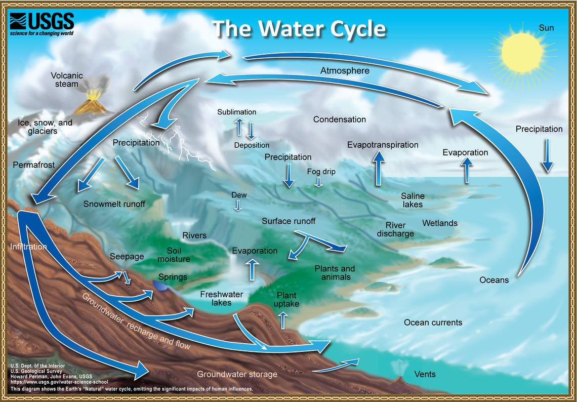
Figure 1. Credit Howar Perlman. USGS public domain.

Flooding happens when the collected water amount is larger than usual. For example, in the case of rivers the volume of space in the riverbed is usually enough for the water to be contained within the river banks. When for some reason – heavy rain fall, accumulation of large amounts of water from quickly melted snow cover, obstruction in the river bed – a large amount of water accumulates there and surpasses the capacity of the river to transport the water to the sea, then flooding occurs.

Flooding in Ostrobothnia

Flooding in Ostrobothnia is a regular and a well-known phenomenon. Floods happen here usually during the spring and the scale of the flood is closely related to the amount of snow in the ground during the winter, the speed it melts and the amount of rain. Spring rain can create flood risks as the ground has usually already absorbed water up to its capacity during the rains in the fall. Melting and moving ice in the rivers can also create ice dams, which can result in local flooding.

Floods have a long history in Ostrobothnia. They are a recurring phenomenon in the area, with thorough historical data recorded. Additionally, during the years there has been extensive work conducted in the area to mitigate the floods and the damages they create. These systems include artificial lakes, corrections in the paths of the rivers and the increased heights of the river banks. Floods still occur and affect the daily routines, but catastrophic events of the old days do not occur frequently. In the location we featured in our magazine image, the data provided by SYKE shows the river water level changes, in the Figure 2 below.

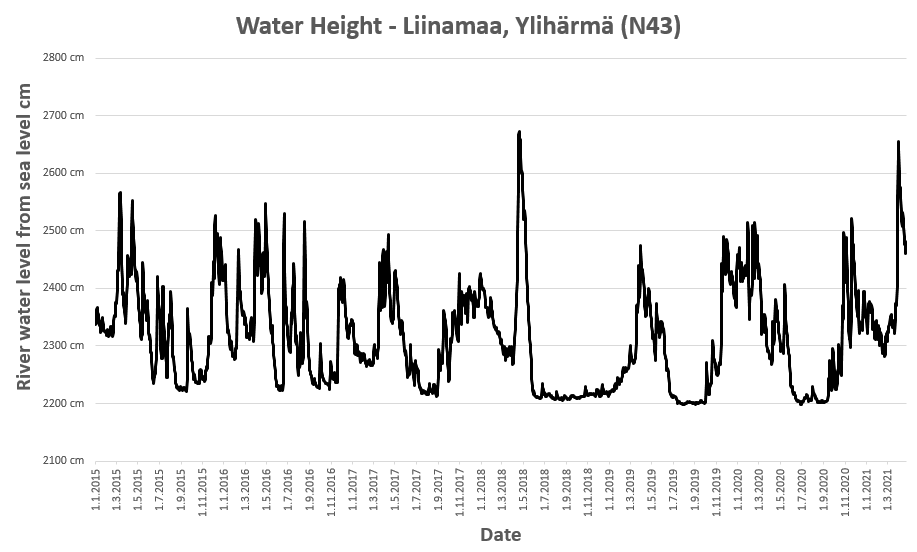
Figure 2. Water level changes 1.1.2015 - 21.4.2021 in Liinamaa, Ylihärmä. Data provided by SYKE.

Important part of the extensive effort to mitigate the adverse effects of the floods is the work of Suomen Ympäristökeskus (SYKE). SYKE produces and updates a collection of information of the current flood situation and the flooding forecasts in “Flood Situation Center” – Tulvakeskus. Additionally, SYKE collects, stores and disseminates a wide array of on the ground measurements. For example, to see the current situation of the area we featured in this month’s image, you can follow this link. As you see, the dataset is quite extensive. In addition to the previous link, you can see an example of the datasets SYKE provides in the following Figure 3. There is depicted the flood area with optical imagery on the right, and left is the extent of an area a flood will cover. SYKE has calculated probability for a flood to cover this amount of land to be 1/100 years. It matches quite closely the observation, so we can very well state that it is an example of an exceptional flood.

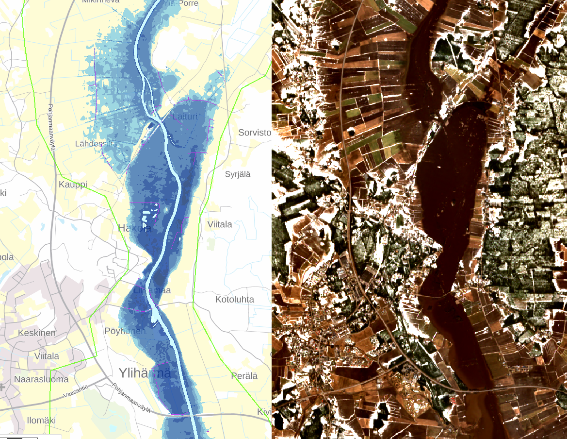
Figure 3. SYKE estimation of an area that a flood with probability 1/100 would cover. Right, Sentinel-2 observation from April 19th 2018.

Flooding and remote sensing

Conceptually, flood forecasting via remote sensing is closely tied to hydrology – a science studying the water cycle we mentioned earlier, water’s properties and how it interacts with the environment. In this approach, remote sensing observations are used as an input part of different calibrated and developed data products, such as products describing stored water balance changes and precipitation. With additional on the ground measurements it is then possible to estimate how the water budget of the water system could be changing and the effects of that change.

Detecting floods with direct observations is more straightforward. Here, the approach is to first detect water, then compare the detected water area to a more normal situation and estimate the difference to see if the situation is a flood.  It is possible to approach the problem from three major directions 1) optical measurements 2) passive microwave instrument measurements or 3) active microwave instrument measurements.

In the first case, the optical measurements, the differentiation is based on the reflectance of the water especially in the near infrared wavelengths compared to soil or vegetation. This is illustrated in the Figure 4 below. The main drawback of the optical classification based comparison are the cloud cover based issues and the inability to function during nighttime. Usually, flooding as an event is such that the response is time critical and if the area is cloud covered, optical measurements cannot deliver the needed information.

Figure 4. Sea water, grass, forest and urban building reflections measured across Sentinel-2 bands.

The second case, passive microwave instruments work as different ground cover emit specific kinds of radiation through the wavelengths and the presence of water changes that. Problem of this approach is that the intensity level of the emitted radiation is very low and to get measurements the instruments have to “look” at larger areas, resulting in resolutions that are not that useful in the cases of local floods.

Third case, active microwave instrument is what we have showcased in the latest article, alongside the two optical measurements. Instrument we used was Synthetic Aperture Radar (SAR) riding onboard of one of the Sentinel-1 satellites.  As you remember, in active sensing the energy to “light” the target comes from the instrument itself (for a quick reminder; see earlier conversations about SAR here and here). As discussed in that earlier article, the surface roughness is one component that affects the intensity of the return signal. Calm water surface returns quite distinctly low backscatter. Most of the EM radiation sent by the satellite is reflected away from the sensor, as you could imagine happening to the light of a flashlight as you’d stand a few meters away from a mirror laying flat on the floor and would point flashlight toward the mirror. Result is that water areas can be identified by that low backscatter, and observations further confirmed by using multiple SAR images.

Below, in the Figure 5, you can see one example of SAR image. In the figure is depicted the intensity of horizontally polarized microwaves – sent as horizontally polarized and received as horizontally polarized. Coloring is based on the measured intensity of the reflected microwave signals after they interact with objects at the surface. Areas with low intensity are colored darker and higher the measured intensity, more bright the pixel. Even visually it is easy to see which areas are water.

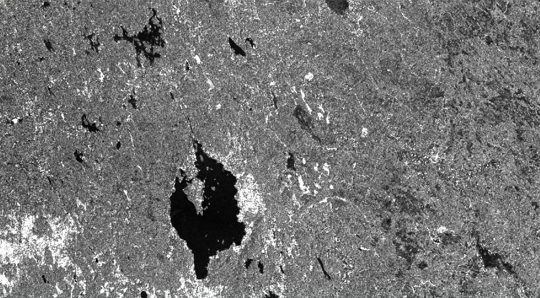
Figure 5. An example Sentinel-1 image.