Pandemic effects on Air Quality

Figure 1. Latest Mega magazine article: change in NO2 mean vertical tropospheric columns before and during COVID-19 measures.

Sentinel-5P and the measuring instrument

This month, we presented in Mega magazine an image (Figure 1) with estimations of air quality. Nitrogen dioxide (NO₂) can act as a useful indicator for air quality. The visualization of the estimations highlighted the differences between the time before COVID-19 outbreak and a period, where most of the restrictions placed by governments were in force. As the majority of nitrogen dioxide sources are related to human activities, these visualizations can be interpreted as an indicator of changes in human activity.

The images are visualizations of NO₂ estimations, and these estimations are based on observations from space. The observations were taken by the European Space Agency’s (ESA) Sentinel-5 Precursor satellite (Sentinel-5P), and by the Tropospheric Monitoring Instrument (TROPOMI) it carries. Sentinel-5P has a sun-synchronous orbit, covers the surface of the entire globe daily and passes over the surface locations in the early afternoon.

The TROPOMI instrument consists of four spectrometers. A spectrometer is an instrument that measures the energy across a range of wavelengths of the electromagnetic spectrum. Each of the four spectrometers in TROPOMI measures electromagnetic radiation (EM) on two bands.  A band is a wavelength range of electromagnetic radiation. These are depicted in the Figure 2 below, where the bands are numbered from one to eight. Some of the bands are in the ultraviolet (UV), some in the visible light (VIS), some in the Near-Infrared area (NIR) and some in the Shortwave infrared (SWIR) ranges of EM radiation. These spectrometers can measure EM radiation from both the direction of the Earth and from the direction of the Sun. You will soon discover why it is setup so.

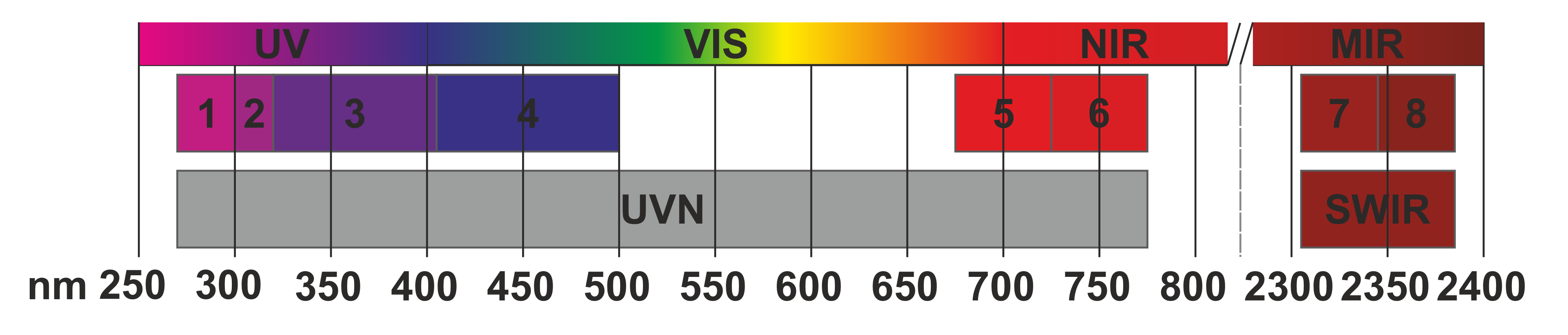
Figure 2. Spectral bands of Sentinel-5P. Source: Creodias.

Differential Optical Absorption Spectroscopy – the basic principles

A simplified way to describe Differential Optical Absorption Spectroscopy (DOAS) is that as light (EM radiation) travels through matter, some of the energy is absorbed. On which wavelengths and how much is absorbed, depends on the matter. If we look at the absorption at many different wavelengths, then we can deduce which matter is absorbing and how much of it is there. The spectral information measured by the TROPOMI instrument is used to estimate amounts of different molecules in the atmosphere with this principle.

DOAS is based on the natural phenomena of selective absorption. EM radiation carries a different amount of energy at different wavelengths. If the energy transmitted at certain wavelength matches the energy gap of the molecules of some matter, then the absorption is more probable. Absorption meaning that the some incoming EM energy is converted in the molecule to kinetic energy. After this kind of absorption, we would notice a dip in the amount of energy carried at that wavelength. Depending on the structure of that particulate matter, it might have several different energy gaps matching different wavelengths, where it is more probable to absorb than in others.

The way the matter absorbs across the spectrum is unique, as the configuration of atoms and electrons is unique to each kind matter. It can be called an absorption profile. For many kinds of matter, these profiles are well known and well measured. Measuring EM radiation precisely at the wavelengths where it is most probable to absorb can tell us two things: 1) if it’s that matter interacting with EM radiation and 2) the amount of the matter, calculated from the energy absorbed.

If we have several types of unknown absorbers, then looking at the measurements at one or two wavelengths do not confirm the type of matter, nor can we calculate the amount of it. The decrease in the energy at a certain wavelength can be caused by any of them, or by some of them. Problem can be solved by examining the lost energies at many wavelengths. If there are enough measurement samples at different wavelengths, then it is possible to calculate how much different unknown absorbers contributed at each wavelength. Based on that, the amount of these unknown absorbers can be calculated. These results can be put in further use as well. For each unknown absorber, the contributions at each measured wavelength can be fitted to the absorption profile to identify the matter.

To summarize, and leaving out the equations themselves. To estimate the density of a matter in a certain path of EM radiation, we need to have five things in principle. First, the original intensity of the radiation at wavelength, as the absorbed amount of radiation is related to the original radiance. Second, the length of the path of the radiation. Third, the absorption probability of the absorber at wavelength (absorption profile). Fourth, the decrease in intensity at that wavelength (the amount of energy that the matter absorbed). And finally, Fifth, if there are several potential absorbers, the decreases in intensity in many wavelengths.

Practice with satellite based DOAS gets a bit more complicated

However, doing this kind of measurements in the real world has effects making it a bit more complex. The original intensity, the length of the path for the EM radiation, and the mixed nature of the atmosphere all require different approach than if it were done just in a laboratory.

First, the initial intensity, usually in the real world the EM radiation originated in the Sun, is not known. It might be a bit surprising considering the spectra of the Sun has been intensively studied and measured. However, before the EM radiation arrives from Sun to Earth, it has already interacted with various molecules in the solar atmosphere, which is not static. This results in absorption at different wavelengths, depending on the molecules and their amount in the solar atmosphere. In addition, there are changes in the EM spectrum related to the movement and rotation of the Sun and the solar cycle.  Luckily, the need to know the initial intensity can be bypassed by using two different paths for the radiation.

Satellite instruments are quite well suited for this, as from the orbit they can observe EM radiation coming directly from the Sun. As result, we have two measurements for two different paths for a certain wavelength. No Earth atmospheric absorption at all, in the one directly from the Sun, and with the atmospheric absorption included in the other. In the equations, the need to know the initial intensity cancels out. We can just look at the ratios. This is why TROPOMI is designed to measure both to the direction of the Sun and to the direction of Earth.

The second problematic area in the real world is the path the EM radiation took. As you remember, the EM radiation comes into the atmosphere, scatters and absorbs there, and reacts with different aerosols, and interacts with something on the ground. Some of it can be reflected back through the atmosphere, where another round of interaction happens, and only then reaches the satellite sensor. Very many things can happen. If we consider EM radiation that travelled this exact path, ending in the satellite sensor, a “ray” A.  The measurement in the satellite sensor at any given point in time consists of this ray A and other rays.

Ray B could be something, which reflected off the upper layers of the atmosphere and travelled a different path, still arriving to the sensor at the same time. There can be very many rays, each with distinct paths. It cannot be determined what exactly was the path each “ray” took and how many of these different paths were. Instead, an effective path is used, which is an estimate and a generalization of all the real paths the “rays” took.

The effective path length is estimated with radiative transfer models, which simulate how EM radiation is scattered and absorbed in the atmosphere. These models are based on the latest understanding of physics and atmosphere. The models use information about the atmosphere at the time of the measurements and additional information such as the known positions of both the Sun and the satellite.

Third consideration related DOAS application in the real world, is the mixed nature of the atmosphere. In a laboratory, it is possible to create a certain length path for the radiation, where the path contains just a certain concentration of certain molecules. Additionally, an EM source can be used, where the initial intensities are known for all wavelengths. In fact, setups similar to this can be used to measure and to record the distinct absorption characteristics of molecules in different wavelengths for further use.

However, in the real atmosphere, concentrations are not necessarily constant and the paths the EM radiation takes can contain many kinds of different molecules, each with a different kind of absorption profiles across the spectrum. Additionally, larger particles than the molecules, called aerosols can affect the attenuation. Aerosols have mostly natural origins such as sea salt particles, sooth or dust, but come in many sizes and forms. Depending on their structure and size, they can scatter or absorb EM radiation at different wavelengths. Besides the effect on the intensity of EM radiation, aerosols also affect the calculated effective path. Clouds can affect similarly depending on the size of the “droplets” they consist of.

EM radiation attenuation in the atmosphere results also from the electrical properties of those particles, that are much smaller than the wavelength of the EM radiation. In addition, EM radiation is attenuated by the shapes of the particles that have sizes close to or above the wavelength. The measured slant column intensity in a satellite at certain wavelength is a result of all these effects along the simulated effective path. In essence, in the measurements we have the results of the absorptions of several different molecules and various other effects. Some of these other effects can be estimated mathematically, others have to be considered noise and just increase the estimation error.

TROPOMI measurements processing

First, TROPOMI measurements are used in a DOAS process, which is based on the principles as discussed. Comparison measurement for each wavelength is taken daily from the Sun and other atmospheric attenuations are taken in account with estimations. The estimation for the amount of matter in a slant column is done with the aid of absorption profiles. These are similar to one presented in Figure 3, where is depicted the absorption cross-section for NO₂ in the range of wavelengths from 225 nm to 675 nm, at 20.83 degrees Celsius. It tells us the efficiency of absorption on particular wavelength. Similar profiles for different molecules or particles would be different, with the highs and lows on mostly different wavelengths.

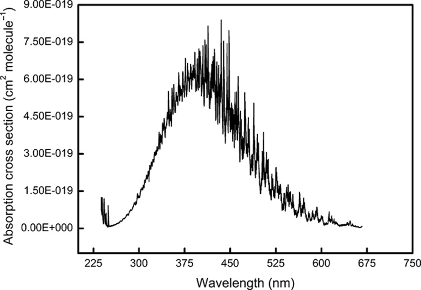
Figure 3. Absorption cross-section of NO2 at 20,85 degrees Celsius. (Source: Vandaele , A. C. , Hermans , C. , Simon , P. C. , Carleer , M. , Cloin , R. , Fally , S. , Mérienne , M. F. , Jenouvirier , A. and Coquart , B. 1998. Measurements of the NO2 absorption cross-section from 42000 cm−1 to 10000 cm−1 (238–1000 nm) at 220 K and 294 K. J. Quant. Spectrosc. Radiat. Transfer, 59: 171–184)

In the TROPOMI NO₂ products, the slant column densities are estimated for NO₂ and some secondary trace gases such as ozone and water. The estimation is based on the principles we discussed earlier, and in addition considering some atmospheric and EM phenomena which we bypassed in the discussion. In principle, estimating the density in a slant column is based on minimizing the difference of the actually measured observations and the modelled explanation for the result. It can be thought of as the actual measurements telling us how right the modelling was. In practice, they are usually very closely matching.

After creating the best solution for the slant column amount of NO₂, the TROPOMI measurements are processed further.  The total slant column NO₂ is separated to the tropospheric and to the stratospheric slant column parts. These parts of the atmosphere are depicted in the Figure 4. The principle is to use external information in the modelled simulations to calculate the stratospheric NO₂ amounts in the areas where is none or very little of the tropospheric slant column NO_{2 .}Then the total slant column amount of NO₂  estimated from the TROPOMI measurements is checked, to see if it is a close match for the simulated value.

By assimilating the total slant column NO₂ in the model, it can be separated in to the stratospheric and the tropospheric NO₂ slant column estimates. Partly the modelling uses values of observations stored earlier, the knowledge and modelling of physical and chemical processes, but also a meteorological model and forecasts for variables such as wind, temperature, surface pressure and others.

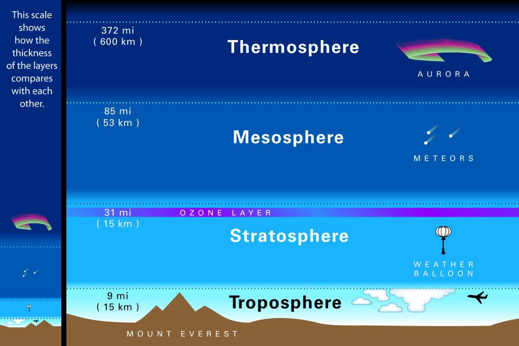
Figure 4. Major parts of the atmosphere. Source: EdMaths.

At this point of the process, we now have the slant column stratospheric and tropospheric NO₂ estimations. Result of the path estimation is usually described as an air-mass factor, which is the ratio between the slant column and the vertical column densities. The slant column, like you remember, is the retrieved measurements in the estimated path, and is estimated with the real world measurements. The vertical column is an imagined measurement describing the densities in a vertical column above a place of interest, for example the air directly above Vaasa, from the surface to the stratosphere.

ESA has created a look-up table based on a model, where the air-mass factors for different altitudes are stored and can be retrieved based on (among others) the solar angles, the viewing angles, the surface and the atmospheric pressures. The modelling for the air-mass values takes in to account the temperature correction for the absorption and the cloud contamination for pixels. The air-mass factors are retrieved for the altitudes that make up the troposphere and summed, and similarly for the stratosphere. Then getting the vertical tropospheric and the atmospheric density column for NO₂ in principle is just a division of the slant column values by the appropriate summed air-mass factors. Now we have the estimates for NO₂ both in the troposphere and in the stratosphere, right above a location of interest.

Nitrogen dioxide

That’s in understandable detail how these vertical column values for NO₂ are produced based on TROPOMI measurements. What can we do with them? What do they mean? We have now information with relative high spatial resolution about the NO₂ estimated amounts above a surface location, in both the stratosphere and in the troposphere, and in a timely manner. Near real time (NRT) products of Sentinel-5P are available approximately 3 hours after the measurement. In short, we can make estimations of an aspect of air quality quite fast, identify sources and examine trends across time globally.

Nitrogen monoxide (NO) is mostly created by human activities, such as burning of fossil fuels (cars, transportation, industry) and the deliberate clearing of forests to cropland by burning. It has natural sources as well such as lightning induced chemical processes, microbial soil emissions or natural forest fires. NO transforms rapidly to NO₂ and vice versa, therefore they are mostly discussed together as nitrogen oxides (NO_x). NO₂ estimations are good estimations for total NO_x as the ratios are understood and how they change depending on the altitude and the temperature.

Both NO and NO₂ react easily with other molecules to produce new combinations, and therefore have short lifetimes. They have short lifetimes especially close to the surface (hours) and longer in the higher altitudes – in the upper parts of the troposphere roughly 1,5 weeks. Seasonal variety affects as well, during winter the lifetime is longer. However, as the lifetimes are short near the surface where the majority emissions happen, most of the detected NO_x can be assumed to be close to the origin.

NO₂ has been linked to health issues and can be used additionally as an indicator of general level of air pollution resulting from traffic, for example. In addition, NO_x affects the environmental processes negatively by being one of the components for the transformations producing the acid rains, contributing to the eutrophication and for producing tropospheric ozone. With these kind of serious impacts, the free availability of quality data products allowing further research of sources and effects is important. With a long series of estimations, it is possible to investigate the local output, output of nations and how well the estimations match what the nations or businesses declare.

Above based mainly on following sources, especially on the lectures by Andreas Richter, Institute of Environmental Physics, University of Bremen.

Babic, L., Braak, R., Dierssen, R., Kissi-Ameyaw, J., Kleipool, J., Leloux, J., ... & Vacanti, G. (2017). Algorithm theoretical basis document for the TROPOMI L01b data processor (No. 8.0, p. 0). Report S5P-KNMI-L01B-0009-SD.

Griffin, D., Zhao, X., McLinden, C. A., Boersma, F., Bourassa, A., Dammers, E., ... & Wolde, M. (2019). High‐resolution mapping of nitrogen dioxide with TROPOMI: First results and validation over the Canadian oil sands. Geophysical Research Letters, 46(2), 1049-1060.

Richter, Andreas. Introduction to Measurement Techniques in Environmental Physics, 2006. University of Bremen.

Richter, Andreas. Nitrogen Oxides in the Troposhere. Sources, distributions, impacts, and trends. Lecture at the ERCA 2010, Grenoble.

Van Geffen, J. H. G. M., Eskes, H. J., Boersma, K. F., Maasakkers, J. D., & Veefkind, J. P. (2019). TROPOMI ATBD of the total and tropospheric NO2 data products. DLR document.

Van Geffen, J. H. G. M., Boersma, K. F., Van Roozendael, M., Hendrick, F., Mahieu, E., De Smedt, I., ... & Veefkind, J. P. (2015). Improved spectral fitting of nitrogen dioxide from OMI in the 405–465 nm window. Atmospheric Measurement Techniques, 8(4), 1685-1699.