Making forest maps using space data and field observations in Sweden and Finland
Published Image. Please click to enlarge.
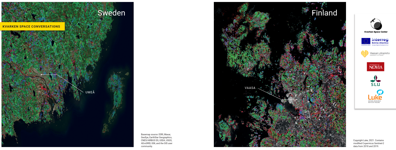
In the Kvarken Space Conversations this month, we had external guest partners who presented the state-of-the-art forest inventory data estimations from both Sweden and Finland. The data and the images were composed by expert organizations in both countries, by the Swedish University of Agricultural Sciences (SLU) and the Natural Resoures Institute of Finland (Luke). In this extended version, we’ll take you through in an understandable level why and how these products were created and what kind of processes are involved in such efforts. Mostly, all discussion and details are based on the documentation provided by both SLU and Luke, for which you find the links at the end and in the Kvarken Conversations page. References are not provided within the text for readability reasons, as the sources are the same for the whole web-article. Exceptions are the images used.
Goal of this extended article of the latest Kvarken Space Conversations is to provide you with an understanding of the general level of the whys and hows of such efforts. We hope to leave you with a comprehension of the types of datasets used and the processes themselves. For the really interested in the details, please refer to the linked articles and report. If you wish to have direct contact with the experts in either SLU or in Luke, drop us a line and we are happy to provide the contacting details. Please also note, that in the Mega magazine the published image around Vaasa was from the latest product by Luke (2019). The discussion in this article about the details on Finnish side is based on the latest published report of the Finnish product, which documents the similar product from year 2015.
Background
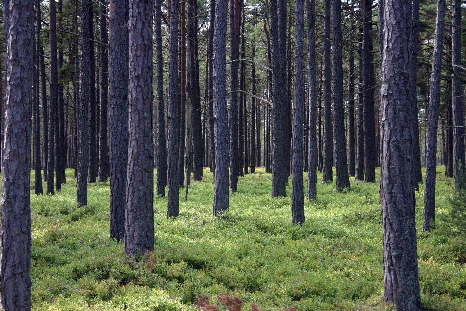
Figure 1. Forest in Stockholm region. Image source: FreeImages / Mikael Cronham. Click to enlarge.
Forest covers large parts of many countries. Especially so in Finland and in Sweden. Forest itself has been a vital part of the lifestyle, beliefs and the traditions in these countries. Even though large areas have been cleared for agricultural purposes during the centuries, the forests have provided a rich variety of resources for gatherers, meat and fur for the hunters, firewood and, in more recent times, acted as a source for a variety of products such as tar, lumber, and paper related products. Currently, many of these uses are still practiced to varied degree, but new important aspects of forest utilization have arisen. Modern important aspects of forests include recreational usage, forests’ contribution in storing carbon, upholding biodiversity, and the environmental protection that the future generations can also see and experience many different types of forests, especially such which are relatively free of the human interference.
Given the importance of forests in the both neighboring countries, it is rather surprising that it was as late as 1900s that systematic and comprehensive forest inventories were started. First National Forest Inventory (NFI) in the world was conducted in Norway 1919 as there were concerns about the sustainability of the forest usage levels. In Finland, the first one was conducted 1921-1924 and in Sweden the first one started in 1923.
However, 1980-1990s new needs started to emerge for more accurate, more localized and more up-to-date information about the state of the forests. The utilization of the forest had risen and new practices emerged in the forestry industry. As the National Forest Inventories take a relatively long period of time to conduct and the required field work would have been prohibitively expensive to create them in a faster cycle, other solutions were devised. In Finland, the first Multi-Source NFI (MS-NFI) was conducted 1990 in the region of Pohjois-Savo, during the 8th Finnish NFI (1986-1994). In Sweden, the first estimated inventory operating on similar principles as in Finland, was started in 1992 and concentrated on the Västerbotten region. The first nation wide results were published in Finland in 1998 and in Sweden in 2000. In Finland, the result product is called MS-NFI and in Sweden, the equivalent product was first called “kNN Sweden” and currently “SLU Forest Map”.
Products in both countries operate on similar principles. Key data components are still the NFIs of conducted in both countries, satellite and in some cases, aerial imagery, and the various digital datasets and for 2015 map in Sweden the tree canopy height. Final forest variable estimations are a product of combining the various data sources and utilizing an interpolation method. Next, let’s take a look at what kind of datasets are used and how, in both countries.
Field Measurements
In both countries, field data estimates are based on round sample plots. The field measurements are usually conducted by a two person team, where other measures the trees and the other person is evaluating other stand attributes. To keep the field measurements proper and comparable between different years and personnel, very detailed guidance is provided for the field workers. In Finland other measured stand attributes consists of things such as land class, topographic class, thickness of the organic layer, development class, dominant species, damages, conducted forestry operations and very many others. Measurements relating to the trees within the circular area in the plot consists of a person standing in the center of the plot and measuring of the trees that are within certain distance from them, in any direction. In Finland, since the NFI 12 the distance where the tree is measured depends on the diameter of the tree, thicker trees being measured from further away than the slimmer trees. A set of measurements are made from the selected trees. A subset is selected as sample trees and more measurement are made from those trees. An interesting tool called Relascope makes this angle count process possible. Relascope is presented in the Figure 2 below. The device was developed by Dr. Walter Bitterlich in 1955. For more information, please see official manufacturer link here. Many variables are also recorded for other stands, if there are others within the circular sample area.
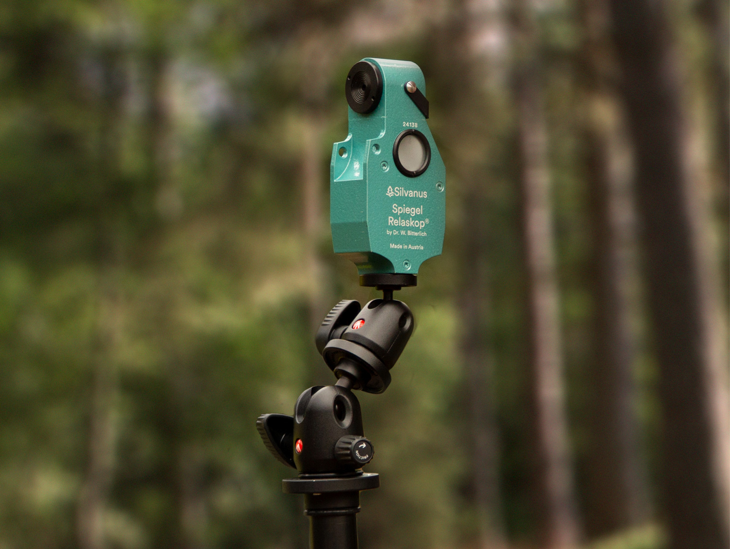
Figure 2. Relascope. Image source: Silvanus. Click to enlarge.
In both countries, the forest variable field data is based on assessing the sample plots during the NFIs. In Sweden, SLU is the organization responsible for carrying out the NFI, and in Finland it is Luke. For the field data MS-NFI 2015 was based on, Finland was divided into 6 regions, where these sampling plots were distributed. In general, in the southern parts the sample plots were more close to each other and distances between them grow larger as we get further north.
For the southern parts of Finland, the distribution of the sampling sites depends on repeating blocks. Each block consist of clusters, and each cluster of varied number of sampling sites. Clusters can be temporary, meaning they can be moved between different NFIs, or permanent when they cannot be moved. In each area the blocks are then repeated over the area, the distance of blocks varying with 12-20 km. Additionally, in the northernmost parts the data is collected more seldom, while in the south a fifth of the sample plots are observed each year.
In Sweden, the sampling covers also the whole country and consists of circular sample plots arranged in to clusters. These clusters are called tracts, where the sample plots are arranged along the sides of a square. Side-length of a square varies between 300m – 1800m and some of the tracts are permanent, and some temporary. Permanent tracts are measured every 5th year. Similarly to Finland, the density of tracts is highest in the southern parts of Sweden and the sampling intensity decreases towards North. This organization of the sites and the frequency has been the same since 2003.
Other datasets
In creation of the estimations several other data sources are needed, besides the satellite observations or the field data. These can be utilized to define the areas of interest for the estimations, to improve the accuracy with information about the soil structure, provide area borders for computing the estimates in more localized scale or in the case of digital elevation models (DEMs), they can be utilized to correct the spectral reflectance based on the slope and sun angles.
In the Finnish MS-NFI 2015, topographic database from National Land Survey (NLS) was used and the main goal was to extract information to help either in delineating the forest areas or to gain additional information about the marshy soil types. Some elements such as roads, power lines and building elements were extracted with buffer zones. Soil type was important information, as even if the growing forest type is the same on a plot, the spectral information can differ if the soil is of different type. Additionally, some of the peatland types cannot be differentiated from mineral soils with remote sensing. Besides the topographic information, information about the protected areas and the administrative borders was retrieved from datasets by Suomen ympäristökeskus (SYKE). Main reason for retrieval of the protected forests was to help in the estimation of the local area wood supply. In Sweden, the topographic information by the Swedish National Land Survey is used, along the same principles. In the Swedish 2000 dataset, topographic information in 1:100 000 scale was utilized to create a forest mask to remove the non-forested areas from the analysis.
DEM data was used in Finland for mainly two purposes. First, to gain the maximum vertical distance from a pixel to its nearest neighbors which can affect the analysis, for example in the cases of cliffs. Secondly, to perform corrections in the satellite observations. The amount of returned reflectance from the surface depends among others things the angle of incoming electromagnetic (EM) radiation and the slope on the surface. With the knowledge of slopes and the sun angle at the time of imaging, corrections were performed. In Sweden, for the 2000 SLU Forest Map, DEM was utilized for terrain shadow correction. Additionally, for SLU Forest Map 2015, DEM was utilized in the creation of tree canopy height data.
Additionally in Finland, coarse large area forest resource data estimations were used. These are based on the data in the previous or the currently on-going NFI, and produced in-principle with a similar interpolation method we will describe in the next part. In Sweden, the national ALS program has resulted in another set of forest maps, Skogliga Grunddata, which is created in co-operation between SLU and the Swedish Forest Agency. Even though it employs a bit similar methods, and has higher accuracy, it presents the state of the forest at the time of the laser scanning for each area unlike the Swedish and the Finnish products discussed, where the estimates of all areas are for the same point in time, across the country. However, the results of the ALS campaigns, the mentioned DEM based on laser scanning, was utilized in the creation of important additional data source, the tree canopy height data. This dataset was produced by the Swedish NLS with stereo-matched aerial images. However, the interior of the northern parts of Sweden was left out from the SLU Forest Map for 2015 as the quality of tree canopy height data was not sufficient. The inclusion of the dataset improved overall accuracy.
Satellite data
In both countries, different satellite data have been used during the years. Aerial images have also been utilized. In Sweden for the SLU Forest Map 2000 data from NASA’s Landsat 7 satellite’s Enchanced Thematic Mapper Plus (ETM+) instrument was used. ETM+ has 8 bands and bands with 30 m spatial resolution were utilized. Bands used for the SLU Map 2000 estimations were visible red, short-wave infrared and two mid-infrared bands. These observations were precision corrected by the Swedish National Mapping Agency.
In the SLU Forest Map 2005 and 2010 observations from the French-Belgian-Swedish SPOT-series of satellites were used, High-Resolution Visible (HRV) and High Resolution Geometric (HRG) instruments with spatial resolutions from 10 m -20 m (multispectral and short-wave infrared). For the SLU Forest Map 2015, observations from European Space Agency’s (ESA) Sentinel-2 constellation were used, provided by the Multispectral Instrument (MSI) onboard the satellites.
In Finland, for the MS-NFI 2015 requirements for the satellite images were large coverage, good availability, multispectral, reasonably priced or free. During that time Landsat-8 was best suited with its Operational Land Imager (OLI) sensor with 9 bands in the area of 435 nm to 2290 nm, with the relevant bands offering 30 meter pixel size. Additionally, during that time the very recently launched Sentinel-2A MSI data was utilized from one overflight.
Spatial accuracy of the Landsat-8 images over Finland was not deemed high enough, and the images were corrected with a process utilizing suitable control points in the imagery. For the Sentinel-2 to accuracy was good enough and only projecting the data to local map projection was required. In both countries, from the satellite images cloud-free mosaics were created with nation-wide coverage. Cloud masking was conducted manually in Finland and semi-manually in Sweden.
In Figure 3 below, (Mäkisara et al., 2019) is illustrated from left to right data sources from: a) acquired Sentinel-2 satellite image, a composite of the three bands in the visible area of EM spectrum b) Representation of the topographical data sources utilized in MS-NFI 2015 map. Note: contains data from National Land Survey of Finland topographic database 4/2016 c) MS-NFI 2015 map of total volume (m3 / ha) with other land use data.
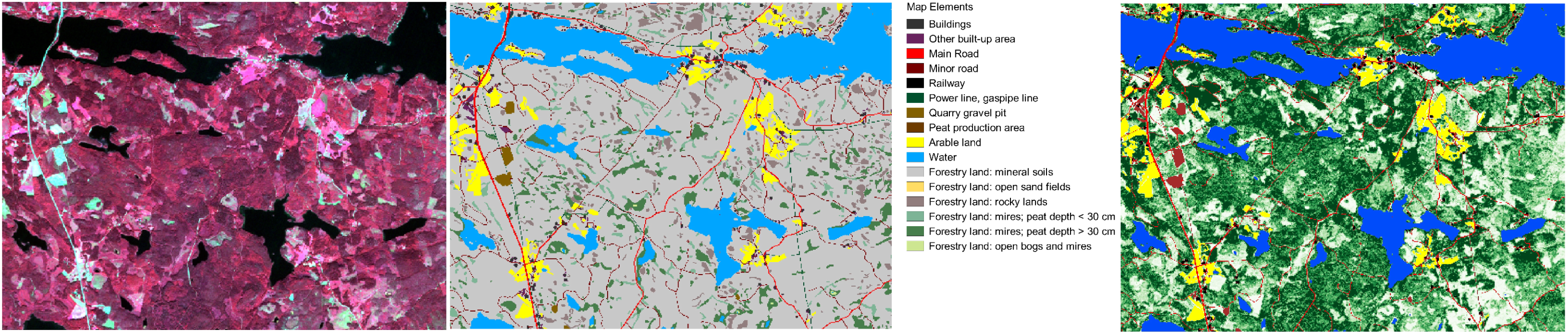
Figure 3. Left to right: 1) acquired Sentinel-2 satellite image, a composite of the three bands in the visible area of EM spectrum 2) Representation of the topographical data sources utilized in MS-NFI 2015 map. Note: contains data from National Land Survey of Finland topographic database 4/2016 3) MS-NFI 2015 map of total volume (m3 / ha) with other land use data. Click to enlarge.
Field Data updating and growth models
A common problem shared in Sweden and in Finland is the temporal mismatch between the field measurements and the satellite imagery. For the estimation products in both countries, a target date is chosen which the variables of the SLU Forest Map and MS-NFI present uniformly across the country. This creates a few problems. As the field measurements for the NFIs are in both countries continuous multiyear processes, however the target date of presentation for the forest maps is chosen, there is always a problem of time difference with the field observations and the acquired images. For example, on average in MS-NFI 2015 the field data represented situation one year before the images. This is problematic especially if large changes have occurred in between the imaging and the field observation dates on the sample plot. For example, if it has been clear cut.
Therefore, as the target date is chosen, all of the field observations are updated to the target date. Based on the information from the NFI field work, proper growth models are selected and applied to the field data. Number of days of the growth season between the field observations and the target date are also calculated. If large changes were detected after the field work and before the imaging, and the change type could be reliably identified, the field parameters were updated to reflect the current situation. If that was not possible, or the change was after imaging but before field work, or there was some other problem with the observations, the plots were omitted.
Estimation process: k-NN
Estimation of the forest variables for the areas without field plots is based on both countries on estimation based on the principles of k-nearest neighbors algorithm (k-NN). Basically, k-NN can be described as utilizing known information in a certain feature space. Unknown variable is then estimated by the known values of its closest neighborghs. These are weighted according to the distance in the feature space. This simple sounding principle is extremely well illustrated by Reese et al. (2003), in the figure 4 below.
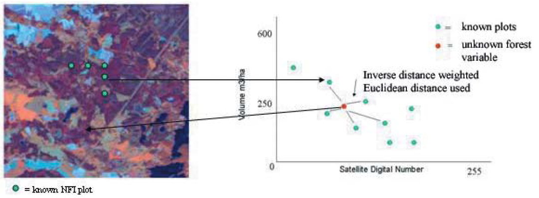
Figure 4. Illustration of k-NN method utilized in SLU Map 2000, image source: (Reese et al., 2003)
For in the image above the variable we are interested in is volume of trees (m3 / ha). For the green points this is known, as they are NFI sample plots. For the red point, this variable is not known. However, for all the points – red and green – the reflected amount of EM radiation is known (digital number) from the satellite observation. Based on the digital number (DN) information, a certain number (called k) most closest points can be examined. Here, k is five, so five sites which spectral information is closest to the red location are picked. Volume for the red point can then be estimated by weighting the volumes of the green points by the inverse Euclidean distance, summing them and dividing by five. Inverse distance means that if the point is farther away (its spectral profile is more different) it contributes less to the average. Similar principle can be utilized for all of the different variables.
That is in general principle how k-NN works in relation to the forestry estimations based on satellite data. In the estimations conducted by Luke and SLU for the national level products, the processes are more intricate, especially in MS-NFI 2015 where the method is now called improved k-NN method (ik-NN). In the both countries, the process has been continuously improved , experimented with and refined during the decades by now it has been used in this context. Please refer to the provided documents for the specifics. They also include more sources for the exact details, developments and rationale of these choices.
Results, and where to get them
Accuracy of the both maps has been improving during the production years and in both organizations, in SLU and in Luke, the development of the methods, models and accuracy is continuous. In both countries, the end result estimations are publicly and freely available. In Finland, the results consist of tabular data and raster maps. Raster maps are easily viewable for everyone for example in the Paikkatietoikkuna, here. MS-NFI datasets are available here.
For Sweden, the SLU Forest Map can be found here.
References, which the article was based on:
Makisara, K., Katila, M., and Perasaari, J. 2019. The Multi-Source national forest inventory of Finland - methods and results 2015. Natural resources and bioeconomy studies 8/2019. Natural Resources Institute Finland, Helsinki. 57 p. Link.
Reese, H., Nilsson, M., Granqvist Pahlén, T., Hagner, O., Joyce, S., Tingelöf, U., Egberth, M., and Olsson, H. 2003. Countrywide estimates of forest variables using satellite data and field data from the National Forest Inventory, Ambio, vol. 32, no. 8, pp. 542–548. Link.
Wallerman, J., Axensten, P., Egberth, M., Jonzén, J., Sandström, E., Fransson, J.E.S., and Nilsson, M. 2020. SLU Forest Map - Mapping Swedish forests since year 2000. In Proceedings of IGARSS 2021, Crossing Borders, Virtual Symposium, Brussels, Belgium, 11-16 July, 2021, pp. 6056-6059. Link.