Managing the Planet's Forests

Figure 1. Published Image.
In this month’s printed article, we displayed (Fig 1) some interesting results from the usage of Forestry Thematic Exploitation Platform (F-TEP) and especially from the usage of AutoChange tool developed by VTT. The tool was used to discover clear cuts done between two Sentinel-2 observations near Vaasa. As the magazine space is rather limited, here in the web extension we would like to take the opportunity to introduce F-TEP and the tool in more detail. Many of you might not be aware of it, but the Sentinel-2 satellites and F-TEP are also very closely related, via the Copernicus programme.
Copernicus
The EU’s Copernicus programme is extensive and has many facets. It’s a large, long-term investment by the EU to provide (for public access) the benefits of space observations. It’s managed by the European Commission and run in partnership with EU member states, European Space Agency (ESA) and various other European organizations. If you have been following the previous Kvarken Space Conversations, you are already a bit familiar with the Sentinel satellites and their observations. Sentinel satellites are also part of Copernicus, they serve as dedicated space assets for the programme. Besides the Sentinel satellites, the Copernicus programme utilizes space observations from the many partnering satellite missions by different countries and organizations. Additionally, the programme collects many different kind of observations done in the Earth. These are measurements done in the location of the phenomena of interest, for example water or air quality measurements. These are known as in-situ observations and in general they are utilized along side the remote measurements from space. In-situ measurements can be used to calibrate the remote sensing observations to estimate derived products or for additional information. The Copernicus programme collects in-situ information from many existing observation networks in the member states.
Even though observations from Sentinel family of satellites are directly available for many use cases, one goal of the Copernicus Programme is to make this extremely large amount of collected remote sensing and in-situ data easily accessible. Additionally, one goal is to enrich the space observations and the collected in-situ measurements by processing them and to offer easy access to the datasets created from this information. These combined datasets are available from the Copernicus services, which have been created for six different application areas: Atmosphere, Marine, Land, Climate Change, Security and Emergencies.
As the understanding of the potential benefits of the space observations and their applications in several different economic or scientific areas grew, and the technological advances leading to the widespread uses of the cloud-based platforms ,it became evident that cloud based processing platforms for satellite images were needed. The Copernicus programme has a cloud based solution for this, the five competing Data and Information Access Services (DIAS) run by different operators. DIAS allow the users to access, manipulate and to download the Copernicus data and information, from the Copernicus Sentinels and from the Copernicus Services, as well as the possible additional information and data from different providers. DIAS are flexible and offer a variety of cloud-based tools and possibilities to build your own workflows.
ESA has approached the similar goal of simplifying the workflows when working with the remotely sensed data first with the Exploitation Platforms (EPs) initiative. Similarly to DIAS, the goal is to remove the need for individuals and organizations to transfer the data to the tools on their own computers. Instead, the platforms should support customization of the workflows and data sources so the need to transfer the same data several times is removed. The Thematic Exploitation Platforms (TEPs) are the end result of that, each offering relevant data and tools in their application domains and aim to provide the user interface to access the datasets and the processing power of the DIASes. For example, the Forestry-TEP utilizes the datasets and the computing capabilities of the CREODIAS DIAS. Currently, TEPs are in various stages of operation and implementation and there are Polar TEP, GeoHazards TEP, Coastal TEP, Urban TEP, TEP Food Security, Hydrology TEP and the Forestry TEP. Since the TEPS as developed in the cloud, they make it much easier to manage the accessing and processing of these data on national, continental and global spatial scales.
Forestry TEP
F-TEP began with a project funded by ESA in 2015. The goal of the platform is to make it easier for the users to use the data and information collected and created in the Copernicus program, in addition to their own data and other data sources, in the area of forestry and especially in the supporting of the forest ecosystem management and the sustainable forest management. It is a cloud-operated platform, meaning that the satellite data can be searched and worked with various tools without the need to do the processing on your own computer. However, it allows for mixed approach as well and offers wide possibilities for customization and automation, therefore supporting both the novice users and the experts in the field.
We had the opportunity provided by VTT to explore the platform and test out some of the basic functionality and specifically their AutoChange tool. Just to give the general understanding of the of the platform, it’s based on an unified workspace (Fig 2) where data can be searched, saved and processed further with different services. The user interface is relatively intuitive and basic usage, such as we tested, can be achieved quite effortlessly. Results can be achieved quicker than with downloading the satellite data and then processing it on your computer. Benefits of that approach come more evident, when larger spatial or temporal coverage is required and more refined processing workflows are used than in our experiment.

Figure 2. Basic overview of the F-TEP. Click to enlarge.
Besides the basic usage, the platform is quite open for extensions and developers have many options to create services for their own use and for others. Sharing services, collected data, and results further is possible with the platform for different groups. Additionally, the platform is accessible via APIs in addition to the graphical user interface. For further information, and to test it out yourself, please see the F-TEP website [link] and the user manual.
AutoChange tool
We took the opportunity to do some basic tests with the Autochange tool developed by VTT and observed excellent results with our first trials. The algorithm central to this tool is documented in “A Hierarchical Clustering Method For Land Cover Change Detection and Identification” by T. Häme, L. Sirro, J. Kilpi, L. Seitsonen, K. Andersson and T. Melkas and published in Remote Sensing on 2020. The following explanation of the tool is mainly based on that publication. References are left out for readability reasons, except in the case of the images. It does not contain direct quotes.
One of the advantages of satellite observations is their consistency. Especially now with the Copernicus programme, extremely large amounts of data are collected daily, stored and made publicly available. The data access and utilization methods are being constantly developed resulting in platforms such as the F-TEP. The consistency of satellite create possibilities that are not available with the more precise observations done with for example drones and airplanes. Airplane or drone observations are active operations, they have to be flown at the location in contrast to satellite observations where data is observed and downlinked, orbit after orbit, and the process can be automated. As a result, usually only satellite observations are available from a location in long series with similar time difference between the observations. Satellite observations are then very well suited for looking at the type and the pace of the changes on the ground. Analyzing these time dependent remotely sensed data is generally called change detection.
Analyzing the change over a time series is not so straightforward however. For example, in the optical series of images there might be masking clouds, or the observed reflections on different wave lengths could be different because of atmospheric effects, or related to the seasonal changes. F-TEP’s Autochange cannot remove the problematics of clouds, but it is insensitive to the changes with different calibration in the observations or the seasonal differences, as instead of being based on changes in the measured reflection in the pixels, it is based on creating homogeneous clusters and identifiying clusters in the image pair. It tries to identify and locate changes that have occurred between images, first image depicting the area before the change and the second image depicting it after the change. The process is depicted in the Figure 3.
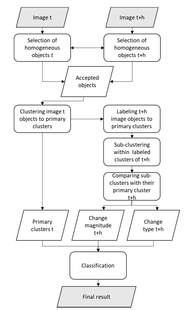
Figure 3. Autochange algorithm. Image source: Häme et al, 2020.
First in both images, candidate pixel areas consisting of relatively similar spectral information are searched for. If the area consist of pixels with relatively similar spectral information within both images, then it’s accepted as a clustering target. These target areas are then clustered in the first image with the k-means algorithm (please see earlier Kvarken Space Conversations, where this was discussed in more detail here), however the spectral information is standardized before the clusterization. The cluster seeds are searched for with an iterative process, where first pixel group in the list is first chosen as the seed. If the next group of pixels is spectrally farther from the already chosen seed, than a parameter which is calculated based on the amount of spectral bands used in the change detection, it becomes the new seed. As the process goes further, other pixel groups need to be spectrally farther than the calculated parameter for all of the already chosen seeds, to be considered a new seed. These clusters are called primary clusters and a result clusterization example is presented in the Figure 4. After the clustering, the clusters are sorted by their “biomass” index, which is approximated with the aid of the reflectance on the visible red area of electromagnetic spectrum. Primary clusters with the highest estimated biomass has then the smallest cluster number and the primary cluster with the lowest estimated biomass has then the largest cluster number.
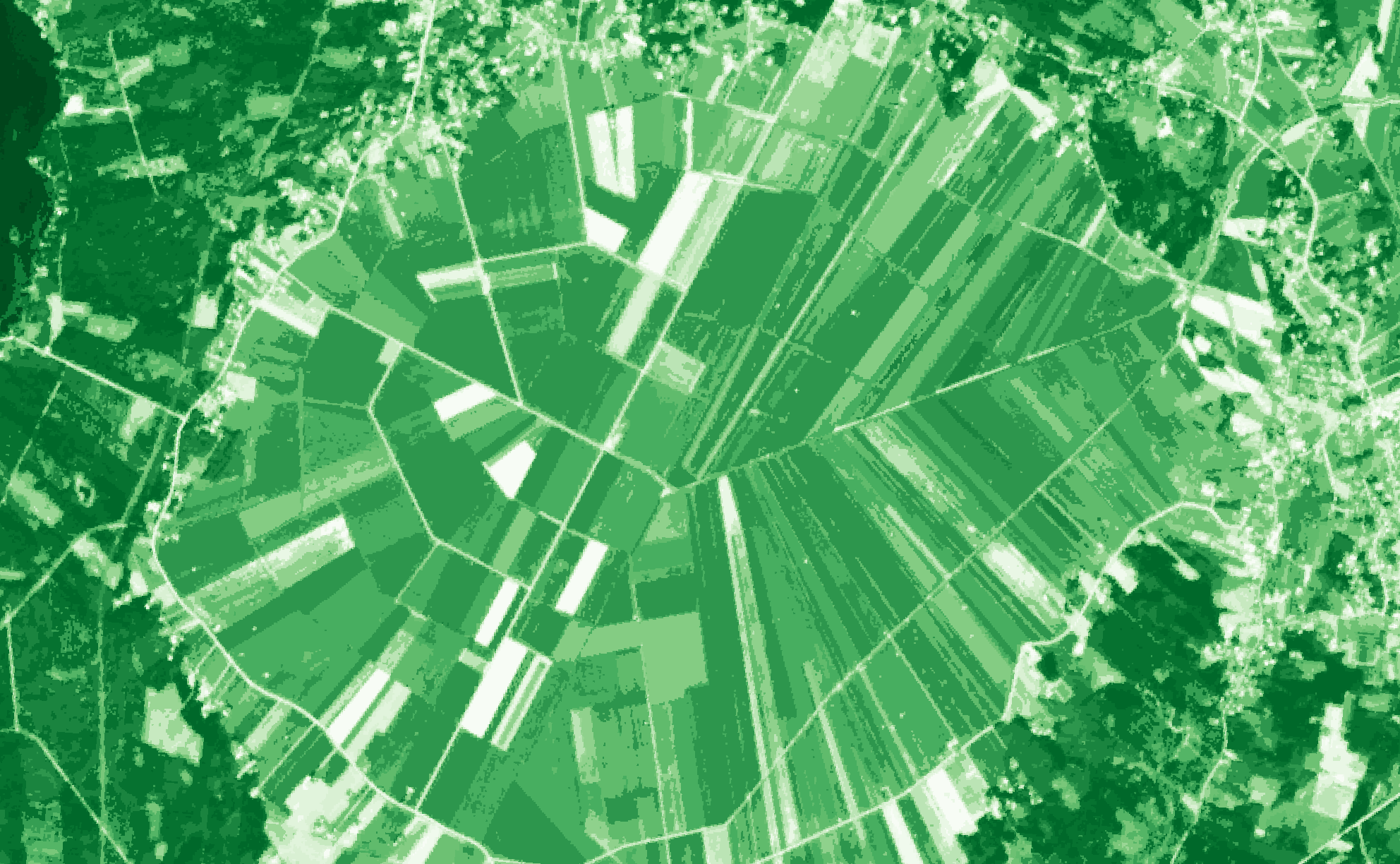
Figure 4. Primary clusters near Söderfjarden. Click to enlarge.
In the second image of the image pair, where the possible change has already happened, the already selected pixel groups are then labeled with the calculated cluster numbers. As the primary clusters were clusterized by the similarity of the spectral profile, if there has been change between the images, it is observable now by the dissimilarity of the spectral information. To investigate and to locate the change, these primary clusters in the second image are now sub-clusterized based on the magnitude of change in spectral reflectances.
Additionally to the area and magnitude of change, the algorithm tries to identify the type of change. That is done with two features based on spectral information. Other is the discussed “biomass” estimate (BM) and the other is the familiar Normalized Difference Vegetation Index (NDVI), which is good indicator for green vegetation and additionally here used as an indicator of the proportion of broadleaf cover. These two features can both either decrease or increase, and the combinations are interpreted as follows in the Figure 5.
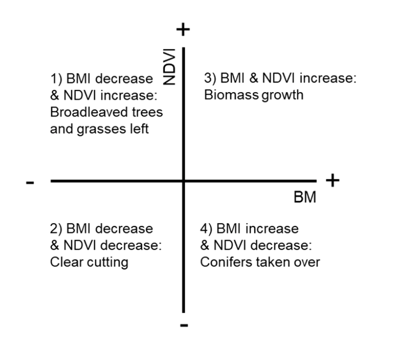
Figure 5. Autochange change types. Image source: Häme et al, 2020.
As a result from this process, for each pixel, we have the primary cluster classification based on the first image, the calculated change magnitude from the second image and the change type based on the BM and the NDVI. Based on this information, which the Autochange tool in the F-TEP provides, we can discover very easily clear-cuts, as displayed in the Figure 6 below.
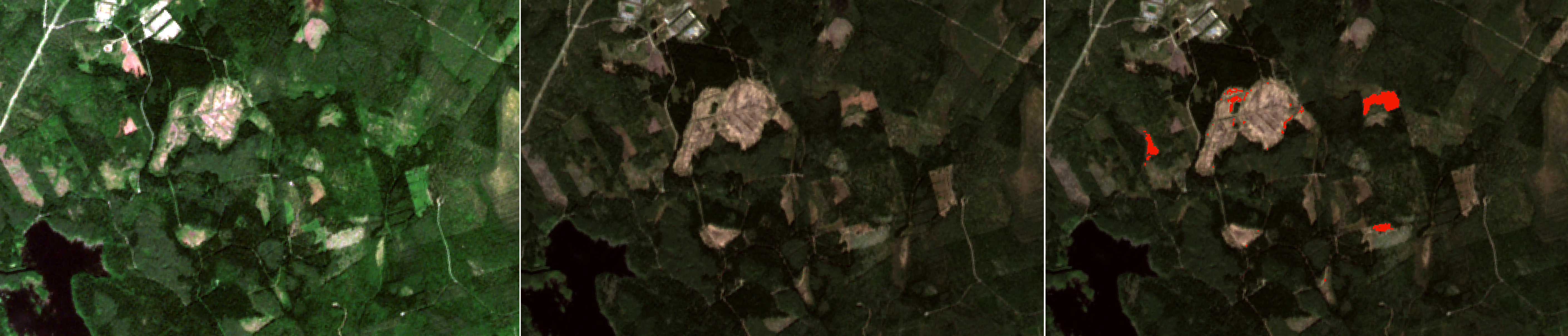
Figure 6. Visualization detail of the AutoChange tool results. Left before image, center after image and detected changes on right. Click to enlarge.
Spruce Bark Beetles
Spruce bark beetles are a major threat for the forests in the Central Europe and with the effects of the climate change they can prosper also in Finland and in Sweden the future. Spruce bark beetle infestations are difficult to monitor as they require normally a close inspection of the trees. To correctly assess the infested area then requires a lot of expensive field work as the infestations can occur in many places at the same time and cover large areas. Additionally, it is very important to discover the infestations and the infested areas as early as possible, to limit the infestations and to harvest the timber in a rescue harvest operation before it’s damaged too much by the pests.
These limitations – the requirement for early detection, large related areas and the amount of field work required make the spruce bark beetle infestations ideal to be identified remotely. There are three different stages in the bark beetle attack. First is called green attack stage, where the tree needles still remain green. Second stage is the red attack, during which the color of the needles changes to yellow and reddish tones. During the third stage, called grey attack, the needles fall and just the bare tree remains. In the Figure 7 below, is depicted an part of an area used in a study (Fernandex-Carrillo et al. 2020) of bark beetle forest damages. All of Sentinel-2 images in the Figure are retrieved with Forestry-TEP. Top row contains an Sentinel-2 image retrieved with Forestry-TEP from year 2020, on left and on right the same area in 2019. Bottom row left is the same area 2018 and on bottom row on right is the area in 2017.
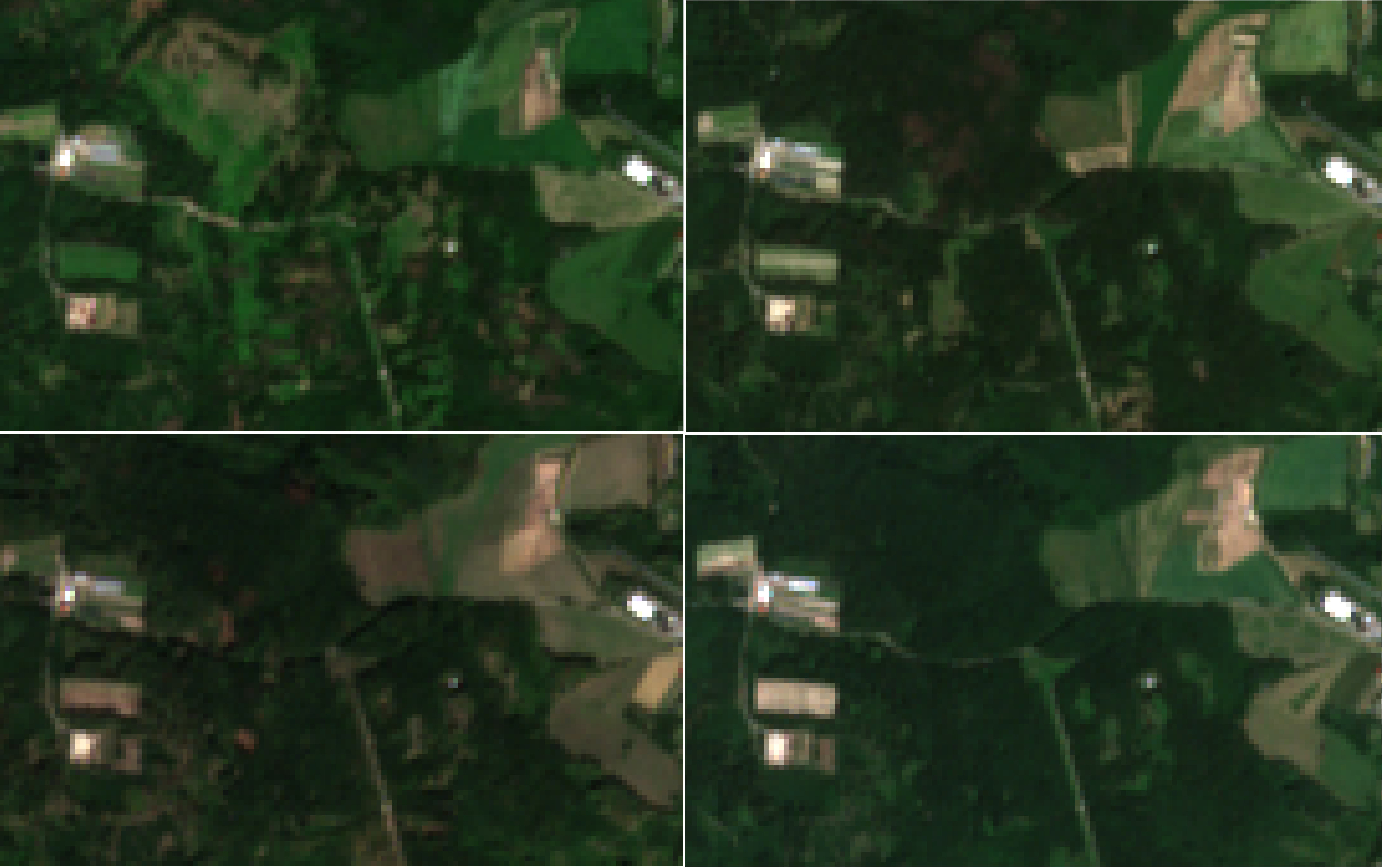
Figure 7. Detail of an bark beetle infested area. 2020, 2019, 2018 and 2017. Click to enlarge.
When looking at the image on the visible wavelengths, it’s quite clear that in the first one from the year 2017 (bottom right corner) things seem quite normal, no visible damages in sight. In the 2018 image (bottom row, left corner) grey attack areas are already visible and in the 2019 image (top row, right corner) large areas are evident. In the 2020 image (top row, left) emergency harvesting has been already done for the infested areas.
Better forecast and indicator of the bark beetle activity can be gotten with different indices utilizing the other parts of the electromagnetic spectrum besides the visible light. You can remind yourself about the indices in a previous Kvarken Space Conversation, here. Fernandex-Carrillo et al. 2020 utilized several different indices based on previous literature. They used the familiar NDVI as an indicator of the plant greenness and photosynthetic activity, normalized difference moisture index (NDMI) utilizing the shortwave-infrared reflectance of water to describe the vegetation water content and green leaf area index (LAIgreen) to estimate the proportion of green leaves in the area. LAI is suitable for looking at indicators of bark beetle existence as the one of the symptoms of later stage infection is the loss of needles. In below in Figure 8, you can see visualization of the differences in these indices.
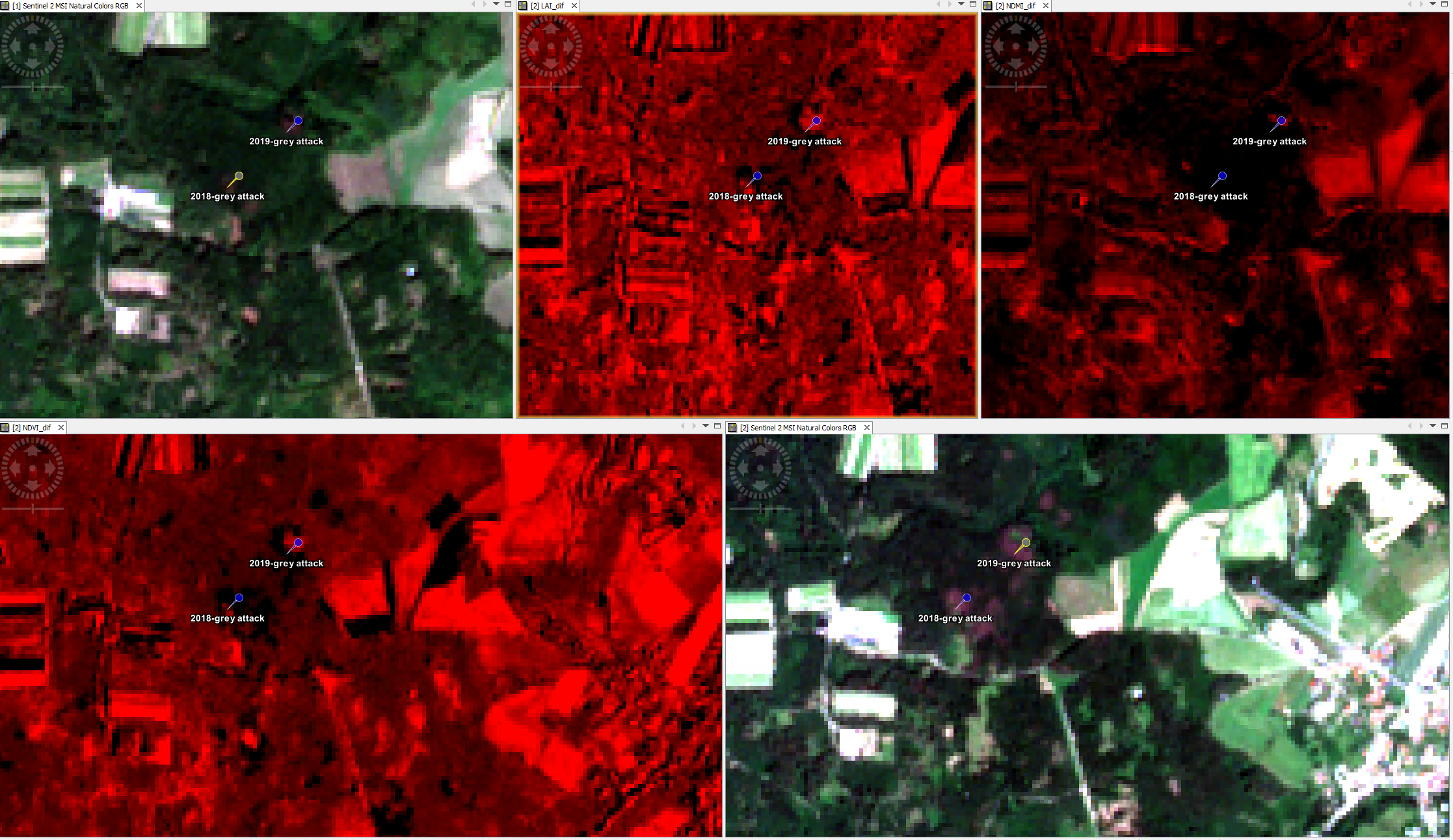
Figure 8. Depicting difference indices. Click to enlarge.
There are other different ways to utilize the multispectral information contained in Copernicus Sentinel-2 images. For example, a recent index developed in the Swedish University of Agricultural Sciences (SLU) (Huo, Persson and Lindberg, 2021) is visualized below in the Figure 9. However, unlike the Autochange tool, which works very well with just two images, the information extracted with these kind of indexes is best utilized with the usage of larger time series of images, to control for seasonal changes as well. To draw conclusions based on the indexes, requires also proper modeling of the results with good in-situ data of the surface cover and information about the bark beetle outbreaks themselves.
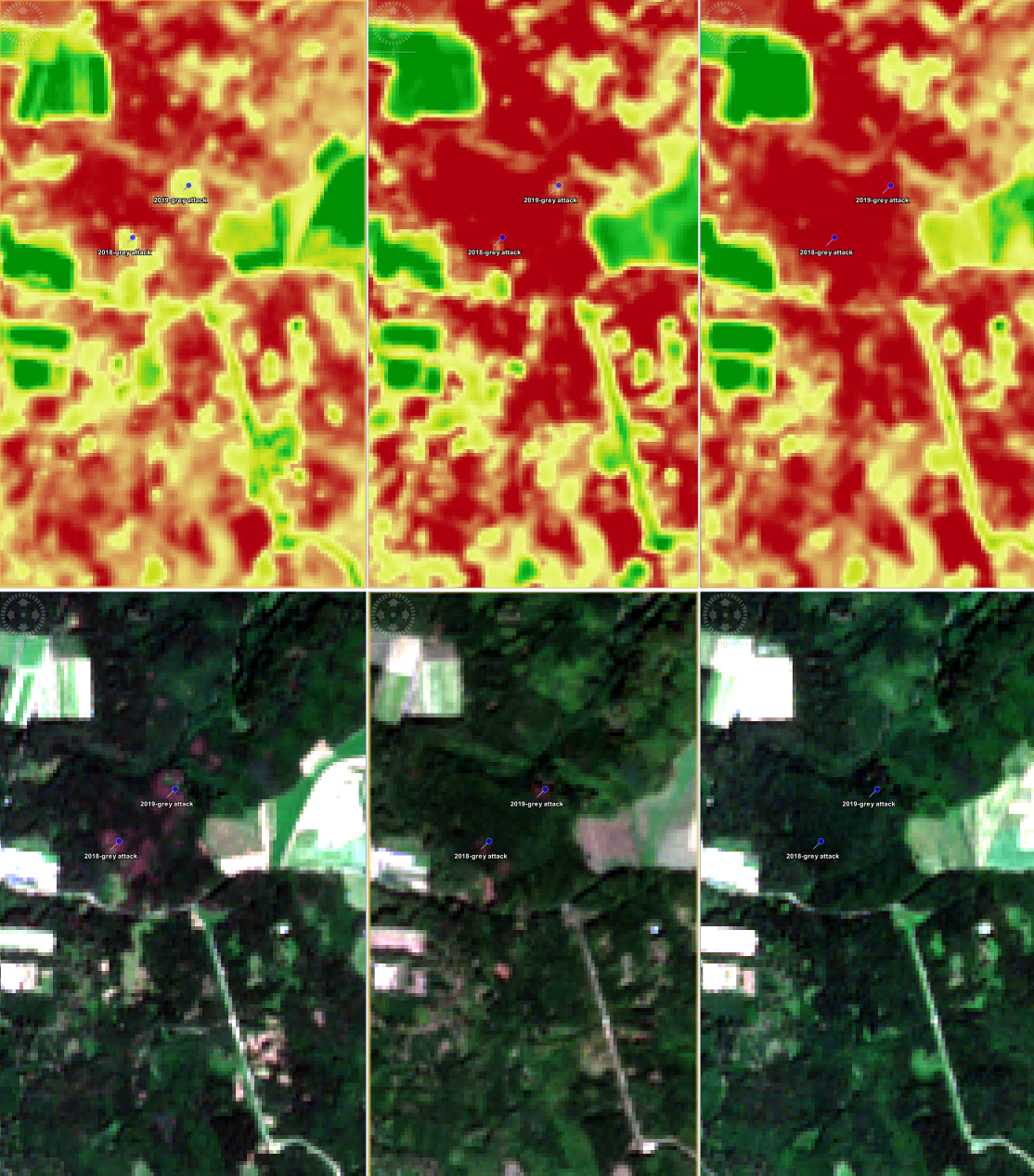
Figure 9. Example of the DRS index developed in SLU. Click to enlarge.
References:
Fernandez-Carrillo, Angel et al. 2020. “Monitoring Bark Beetle Forest Damage in Central Europe. A Remote Sensing Approach Validated with Field Data.” Remote Sensing 12(21): 3634.
Huo, Langning, Henrik Jan Persson, and Eva Lindberg. 2021. “Early Detection of Forest Stress from European Spruce Bark Beetle Attack, and a New Vegetation Index: Normalized Distance Red & SWIR (NDRS).” Remote Sensing of Environment 255: 112240.
Häme, Tuomas et al. 2020. “A Hierarchical Clustering Method for Land Cover Change Detection and Identification.” Remote Sensing 12(11): 1751.